01-Paraver

Background

What is Paraver?

Paraver was developed to respond to the need to have a qualitative global perception of the application behavior by visual inspection and then to be able to focus on the detailed quantitative analysis of the problems. Expressive power, flexibility and the capability of efficiently handling large traces are key features addressed in the design of Paraver. The clear and modular structure of Paraver plays a significant role towards achieving these targets.

Paraver is a very flexible data browser that is part of the BSC-Tools toolkit. Its analysis power is based on two main pillars. First, its trace format has no semantics; extending the tool to support new performance data or new programming models requires no changes to the visualizer, just to capture such data in a Paraver trace. The second pillar is that the metrics are not hardwired in the tool but programmed. To compute them, the tool offers a large set of time functions, a filter module, and a mechanism to combine two time lines. This approach allows displaying a huge number of metrics with the available data. To capture the experts knowledge, any view or set of views can be saved as a Paraver configuration file. After that, re-computing the view with new data is as simple as loading the saved file. The tool has been demonstrated to be very useful for performance analysis studies, giving much more details about the applications behaviour than most performance tools. Some Paraver features are the support for:

1. Detailed quantitative analysis of program performance.
2. Concurrent comparative analysis of several traces.
3. Customizable semantics of the visualized information.
4. Cooperative work, sharing views of the tracefile.
5. Building of derived metrics.

How are Paraver traces generated?

Paraver traces are generated by instrumenting the code with Extrae. This library intercepts the application and collects data such as PAPI counters with minimal overhead. The instrumentation can be done dynamically at certain points such as MPI and/or OpenMP calls. Manual instrumentation by directly calling the Extrae API is also supported. For more information on Extrae, check the official site.

Link: https://tools.bsc.es/extrae

How to run Paraver

Paraver is already installed in the nord3 cluster we are using for this session. You only need to source the configuration file in the current directory and you will able to open Paraver:

$ source configure.sh
$ wxparaver

Important: Remember to enable X-forwarding in your ssh connection to be able to open the Paraver graphical interface.

[Highly recommended] Install Paraver in your local machine

You can download and install Paraver from BSC’s tools-site. Both pre-compiled and source packages are available.

Link: https://tools.bsc.es/downloads

[Optional] Paraver tutorials

You can go through the official Paraver tutorials available in BSC’s tools-site.

Link: https://tools.bsc.es/paraver-tutorials

The Paraver installation in nord3 already contains an embedded version of the tutorials. You can access them through the toolbar at the top of the main window “Help” -> “Tutorials...”.

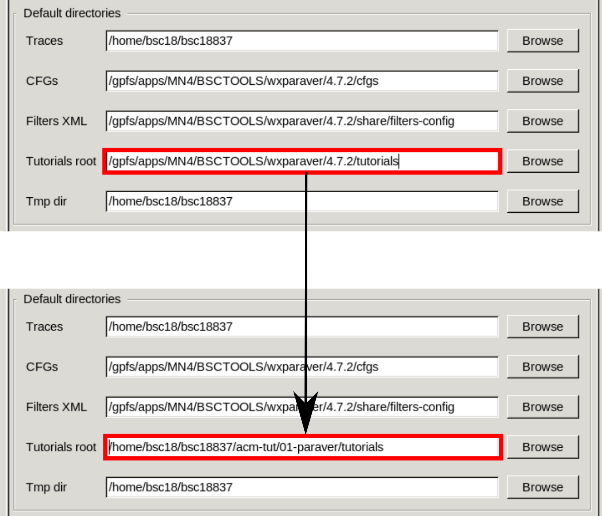
You can also embed this tutorial into Paraver. To do so, go to “File” -> “Preferences...” and change the “Tutorials root” field to point to the “tutorials” directory included in the tar ball that you have downloaded for this tutorial.

Running Paraver for the first time

How to open Paraver

# Set up your environment
$ source configure.sh

# Run Paraver
$ wxparaver

# You can also feed Paraver a trace from the command line
# Replace <mytrace.prv> for the trace that you want to open
$ wxparaver mytrace.prv

# Paraver also reads compressed gzip traces
# Replace <mytrace.prv.gz> for the trace that you want to open
$ wxparaver mytrace.prv.gz

Traces and configurations

A Paraver trace is typically composed by three files:

• .prv the actual trace with records of events happened during execution and the data collected by Extrae
• .pcf information about what type of data has been collected
• .row information about the number and name of processes/threads

The trace files contain information about an execution. Paraver uses configuration files (cfgs) to display the data in different ways. By default, you will find some basic cfgs accessing the Hints menu in the toolbar at the top of the main window. This is the preferred method to load cfgs. The Hints menu will show cfgs that are relevant for the loaded trace. For example: for a trace with MPI, a relevant cfg is the “MPI profile”; for a trace with OpenMP, “parallel functions” and so on.

Navigating through Paraver

Main window

The main window’s purpose is to manage all your loaded traces and cfgs. It is divided into three sections:

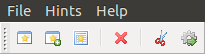
• Top toolbar is located at the top of the window. From this menu you can load and unload both traces and cfgs. The Hints dropdown will display basic cfgs for your current loaded trace. Under Help you can find the tutorials shipped with your Paraver installation.
• Quick access menu is located right under the top toolbar. It gives access to different Paraver functionalities once you have loaded a trace:
  • Open a new window. By default, this window will be configured to show the CPU states. This is NOT the preferred method to load a cfg. You should use the Hints menu or browse through your Paraver files until you find the cfg you want to load.
  • Open a new derived window. Clicking on it will prompt you with a dialog to combine two previously created windows.
  • New histogram. Will create a histogram from the currently active control window.
  • Delete selected window.
  • Filter trace. Clicking on it will prompt you with a dialog to cut and/or filter a trace.
  • Run application. Clicking on it will prompt you with a dialog to invoke other BSC performance analysis tools.

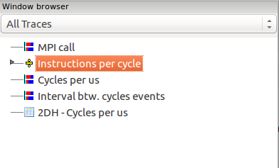
• Window browser contains a list of all the currently loaded cfgs for the active trace. The dropdown menu at the top of the browser displays the name of the active trace. You can switch between active traces by selecting them in the dropdown menu.

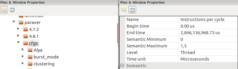
• Files & Window Properties is divided into two tabs:
  • Paraver Files contains a simple file browser to navigate through the available cfgs.
  • Window Properties contains information about the active cfg. You can modify the cfg through this menu. The actual properties displayed depend on the type of active window.

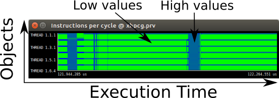
Control views

Control views, or timelines, allow you to visualize metrics throughout execution time. They are structured as follows:

• Vertical axis represents the objects being represented. An object may be an MPI process or a thread.
• Horizontal axis represents time. It is divided in discrete chunks which are called bursts. These bursts are the space betwen two instrumentation points where Extrae has gathered information. This points usually correspond to MPI calls, OpenMP calls or even the user’s explicit calls to the Extrae API.
• Color scale, also known as Semantic scale, represents the metric being measured. Basic metrics are one of two types:
  • Categorical values such as CPU states or MPI Calls. These are displayed with a color code, where each color represents a different state or call.
  • Numerical values such as IPC, Cache misses, Instructions, etc. These are displayed with a color gradient which ranges from a light green (low values) to a dark blue (high values). Values outside the semantic scale are displayed in either yellow (below the minimum value of the scale) or orange (above the maximum value of the scale).

You can navigate control windows to find points of interest of your performance analysis. Here are some tips on how to work with control windows:

• Mark the beginning/end of bursts with flags by right-clicking and selecting “View” and then “Event flags”.
• View the exact value of a given burst by hovering over it and double-clicking.
• Zoom in by left-clicking and dragging the time frame you want to zoom in.
• Undo zoom by typing Ctrl+U or by right-clicking and selecting “Undo zoom”.
• View the whole execution time by right-clicking and selection “Fit Time Scale”.
• Show info panel by double-clicking over the burst you want to analyze. You can also right-click and select “Info panel”.
• Fit the semantic scale to include all values present in the current window by right-clicking and selecting “Fit Semantic Scale” and “Fit Both”.
• A red warning icon will appear in the bottom-left corner of the window if there are values outside the semantic scale. You can click on the icon to fit the semantic scale.

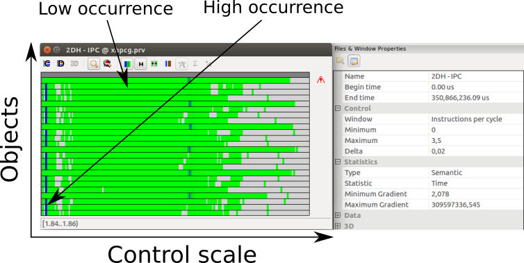
Histograms

Histograms allow you to visualize metrics in a global scope instead of representing them on a timeline. Each histogram requires an associated control window. Histograms can be interpreted as color coded tables of data. They are structured as follows:

• Vertical axis represents the objects being represented. An object may be an MPI process or a thread.
• Horizontal axis, also known as Control scale, represents the histogram’s bins.
• Color scale, also known as Semantic scale, represents the occurrences of the metric being measured. The semantic scale can be controlled through the “Statistics” menu in the main window.

The value of each cell of the histogram represents the time that a given object has spent inside the corresponding histogram bin. This can be changed for other statistics such as the percentage of the execution spent in the bin, “% Time”; or the number of bursts that fall inside that bin, “# Bursts”. Similar to the control windows, the color scale ranges from light green for low values to dark blue for high values.

Here are some tips on how to work with histograms:

• Zoom in a range of bins by left-clicking and dragging to select the bins you want to zoom in.
• Undo zoom by typing Ctrl+U or by right-clicking and selecting “Undo zoom”.
• Open the associated control window by clicking on the leftmost icon in the toolbar at the top.
• Toggle on/off numerical values by clicking on the magnifying glass icon in the toolbar at the top.
• With the numerical values turned on, you can see total statistics of each bin by scrolling to the bottom of the histogram. You can also toggle all the partial statistics by clicking on the summation icon in the toolbar at the top.
• Transpose the histogram by clicking on the “H” icon in the toolbar at the top.
• Hide empty columns (bons with no occurrences) by clicking on the icon to the right of the “H”.

MPI+OpenMP example

In this section we will conduct a very simple study. We will use a trace extracted from an execution of the LULESH benchmark using eight MPI processes, each one with four OpenMP threads.

Load the trace

First, open Paraver and load the trace. You can find it under traces/lulesh_8mpi_4omp.prv.gz.

You can also feed the trace directly through the command line.

$ wxparaver traces/lulesh_8mpi_4omp.prv.gz

Discover application structure

We will now try to identify if there are execution patterns in this benchmark such as an itterative pattern or very distinct execution phases.

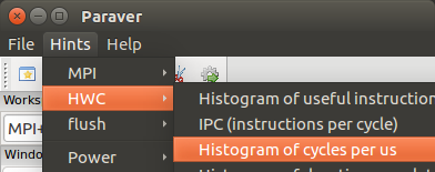
Load the “IPC (instructions per cycle)” cfg under “Hints” -> “HWC”. Zoom in to discover the itterative pattern of this specific benchmark.

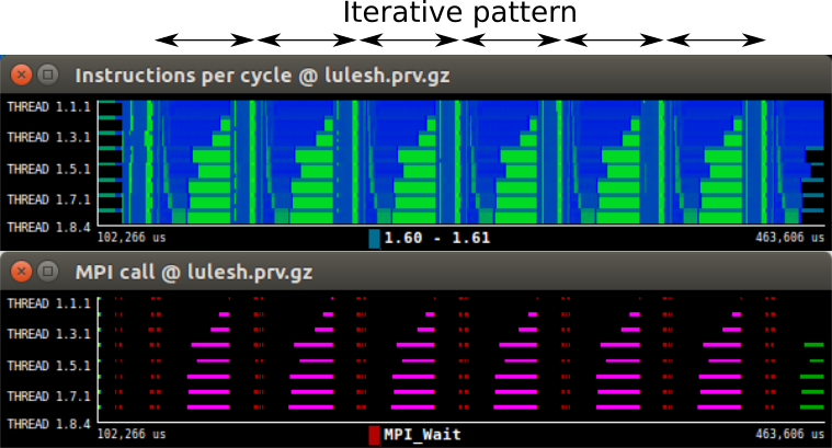
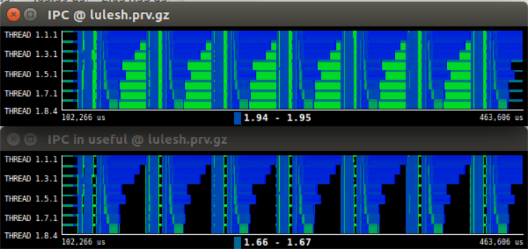
In the image, the pattern repeats six times. It starts with a small blue section, with an IPC around 2.0. It then continues with a very short green section, IPC ~0.45. Then there is a longer section where processes start with a high IPC value (in blue) and then transition to a lower IPC (in green). Note how the blue part has a different duration for each process.

The colors in this cfgs represent different MPI calls. The background color (black in the image) represents outside of an MPI call. There are only six objects that invoke MPI calls. These correspond to the master threads of each MPI process.

Now open the “MPI call” cfg under “Hints” -> “MPI” -> “MPI profile”. You can easily set the same time frame as in the IPC by copying (Ctrl+C) the IPC window and pasting it (Ctrl+V) into the MPI call window.

This new window shows the MPI calls throughout the execution time. Each type of MPI call is coded with a different color. The pattern starts with two sections with point-to-point communications (red bits) and then a collective operation (magenta lines). The black sections identify sections of the execution time outside MPI calls.

Combining control windows

By default, the IPC cfg will show the metric for both computational and communication portions of the execution. To only get the IPC of the useful sections we need to combine it with another cfg.

Browse through the “Paraver files” tab to find “useful.cfg” under “General” -> “views”. This new cfg highlights only the phases where the threads are performing useful computation.

In the window browser, drag and drop the IPC cfg over the useful cfg. A new dialog will appear with options on how to combine the two views. Hit the “OK” button to generate an IPC window which only includes the useful portions of the execution.

CPU states

Click on the “new single timeline window” button to open a default cfg that shows the CPU states of each thread. Copy and paste the time from one of your previous control windows. The CPU states are color-coded.

To quantify how much how much time each thread spends in each state, create a new histogram by clicking on the “New histogram” icon. Toggle the numeric values by clicking on the magnifying glass icon and hide the empty columns. By default, the statistic shown in histograms is the absolute time (ns) each thread spends in a given bin. You can change this statistic in the main window under “Statistics” -> “Statistic” and select “% Time”.

Notice how the “Running” state is actually the state in which the threads spend the most time in (around 90% of the time). Some threads seem to behave differently. The master threads of each process spend less time in the “Running” state.

Load balance

Toggle off the numeric values of the histogram and open a filtered control window by clicking on the right magnifying glass icon and selecting the “Running” column of values. The new timeline shows only the portions of the trace where threads are in “Running” state. We have manually replicated the “useful.cfg” that we loaded earlier.

Notice how Some threads are idling a lot more than other. This is due to a workload imbalance. You can quantify the amount of imbalance by zooming into one of the iterations and creating a new histogram. Then toggle on the numerical values and go to the total statistics at the bottom of the table. The “Avg/Max” metric represents how much work has done the thread that has worked the most in comparison to the average. If this metric is close to one, the more balance the execution. In this case, the balance is around 0.60, which is a very low value.

Delving deeper

There are myriads of metrics to extract from Paraver. Have a look at the tutorials shipped with the Paraver installation for more information. You can also have a look at the POP European project for examples on extensive performance studies.